Solver Mode Benchmarks

benchmarks/solver_modes/ compares SSQP's own solver modes against each other, rather than against other solvers: for a given problem, how does formulating the dynamics equality constraint as ForwardDynamics (torque controls), InverseDynamics (acceleration controls), or ReducedInverseDynamics (acceleration controls, unactuated DOFs propagated implicitly) affect convergence?

This page covers the trajgen/ half of that directory, which benchmarks offline trajectory generation. For each model, many randomly generated problems (different targets, same cost/constraint structure) are solved once per applicable dynamics mode, all the way to --horizon/max-iteration limits rather than stopping at the first converged solve, so that the full convergence trace is available for every problem.

Reading the plots

Each plot aggregates every problem generated for that model, one line per solver mode, against SQP iteration on the x-axis:

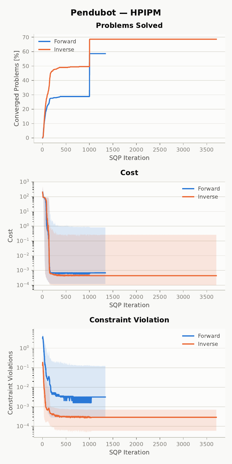
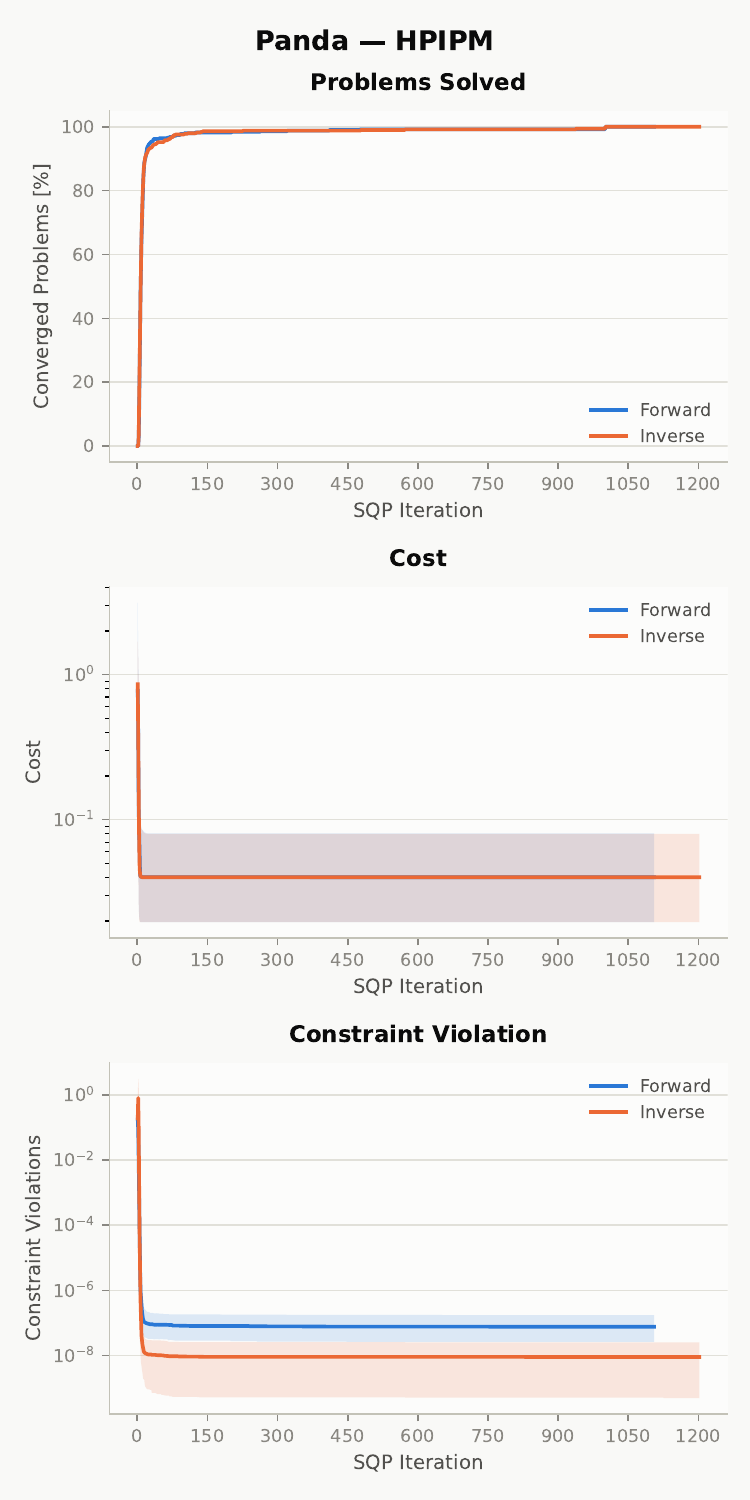
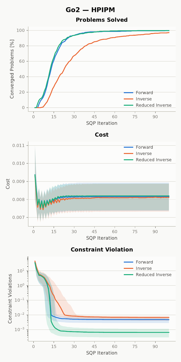
• Problems Solved: the cumulative percentage of problems that have converged by a given iteration. A failed problem still counts toward the total, so it pulls the curve down rather than being excluded.

• Cost: the per-problem worst per-stage cost, log-scaled. The solid line is the median across problems, the band the 25th-75th percentile range.

• Constraint Violation: the per-problem worst per-stage violation (position/velocity/torque/friction bounds and the dynamics-transition defect), log-scaled, against the shared solver tolerance. Median line and interquartile band, as above.

All three plots below use the HPIPM QP backend.

Running the benchmarks yourself

See the solver_modes/ README for full setup. Once set up, from the trajgen/ directory:

python run_benchmark.py [pendubot|panda|go2] -q hpipm

--modes restricts which dynamics modes are run (all applicable modes by default), and -n/--n-problems changes how many problems are generated (50 by default; the Pendubot, Panda, and Go2 plots below were generated with -n 500). Results land in trajgen/data/results; plot.py then renders one model's results into the plots shown below:

python plot.py pendubot -q hpipm

Pendubot

The same Pendubot Swing-Up problem as in the solver benchmarks, run here with a randomized target configuration per problem, comparing ForwardDynamics against InverseDynamics.

Panda

The Franka Panda reaching random targets within its feasible region, comparing ForwardDynamics against InverseDynamics.

Go2

The Go2 quadruped walking to a randomized target pose, comparing all three dynamics modes: ForwardDynamics, InverseDynamics, and ReducedInverseDynamics (which propagates the unactuated floating base implicitly instead of constraining it explicitly).

Go2 Multi Jump

The Go2 performing five jumps in place, landing on a different combination of feet in each gap between jumps (see Go2 Multi-Jump). Unlike the models above, this problem keeps the same fixed choreography across runs rather than randomizing targets, so only a single generated problem is benchmarked per mode; there's no convergence trace to aggregate into a plot, just that one run's runtime, iteration count, final cost, and constraint violation, using HPIPM. Constraint violation is the same worst per-stage quantity described above (bounds and dynamics-transition defect), against the shared tolerance of 1e-2.

Dynamics Mode	Runtime	Iterations	Final Cost	Constraint Violation
ForwardDynamics	257.3 s	936	0.0463	0.129
InverseDynamics	310.5 s	1000*	0.0337	4261.8
ReducedInverseDynamics	47.9 s	174	0.0456	0.253

* Hit the 1000-iteration cap without meeting the solver's convergence criterion.

G1 Jump

The Unitree G1 humanoid jumping vertically in place (see G1 Jump). Same single fixed-choreography problem setup as Go2 Multi Jump, benchmarked with HPIPM.

Dynamics Mode	Runtime	Iterations	Final Cost	Constraint Violation
ForwardDynamics	215.0 s	244	0.7592	0.154
InverseDynamics	37.4 s	46	0.7530	0.198
ReducedInverseDynamics	12.8 s	17	0.7549	0.032